1. Characteristic Polynomial to find eigenvectors and eigenvalues.
   • Characteristic Polynomial of a square matrix is a polynomial which is invariant under matrix similarity and has the eigenvalues as roots (Wikipedia).
   • Trace of a square matrix is a sum of all element in the main diagonal of that matrix.

   • Formula: \(A\cdot x = \lambda \cdot I \cdot x \\ \Rightarrow A\cdot x - \lambda \cdot I \cdot x = 0 \\ \Rightarrow (A - \lambda\cdot I)\cdot x = 0\)

     For vector x not equal to zero —> $A - \lambda \cdot I = 0$ —> $det(A-\lambda \cdot I) = 0$ .

     Notation:

     • Set of n eigenvectors is Eigenspace Ker(A - lambda * I).
     • Dimension of this kernel (Nullspace) is called geometric multiplicity.
2. Eigen Decomposition (ED) and some simple proof approaches.
   • Formula:
   \[P^{-1} \cdot A \cdot P = E\]
   • Notation:
     • P is square matrix whose columns are eigenvectors.
     • A is original square matrix.
     • E is diagonal (square) matrix whose elements in the main diagonal are eigenvalues corresponding to eigenvectors in P.
   • Proof for ED:
     • Let $P = [p_1 \space \space p_2 \space \space p_3, …]$ be eigenvectors of A.
     • Let E be diagonal matrix whose elements in main diagonal are eigenvalues (lambda).
     • We have:
     \[A \cdot P = \lambda \cdot P \\\Rightarrow A \cdot P = A \cdot [p_1 \space \space p_2 \space \space p_3 \space ...] \\ \Rightarrow A \cdot P = [A\cdot p_1 + A\cdot p_2 + A\cdot p_3 \space ...]\]
     • According to definition: $A \cdot x = \lambda \cdot x$
     • Therefore,
     \[A \cdot P = [\lambda \cdot p_1 + \lambda \cdot p_2 + \lambda \cdot p_3 \space ...] \\\]
     • Then,
     \[A \cdot P = \begin{bmatrix} p_1 & p_2 & p_3 & ... & p_n\end{bmatrix} \cdot \begin{bmatrix} \lambda_1 & 0 & 0 & ... & 0 \\ 0 & \lambda_2 & 0 & ... & 0 \\ 0 & 0 & \lambda_3 & ... & 0 \\ . & . & . & ... & . \\ . & . & . & ...& . \\ 0 & 0 & 0 & ... &\lambda_n\end{bmatrix}\]
     • Finally,
   \[A \cdot P = P \cdot E \\ \Rightarrow P^{-1} \cdot A \cdot P = P^{-1} \cdot P \cdot E = E\]
   • Eigendecomposition is also called “diagonalize matrix “—> when we implement ED means that we diagonalize matrix.
   • Conditions for the matrix to be diagonalizable:
     • It must be square matrix.
     • It must contain n eigenvectors linearly independence corresponding to n eigenvalues.
3. Application
   • Calculate $A^n$ (A power of n) —> $A^n = P\cdot E^n \cdot P^{-1}$ (the power of diagonal matrix is the power of all elements in its main diagonal).
   • Find inverse matrix $A^{-1} = P \cdot E^{-1} \cdot P^{-1}$

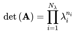
   • Calculate determinant: det of diagonal matrix = product of all the elements in the main diagonal.

     

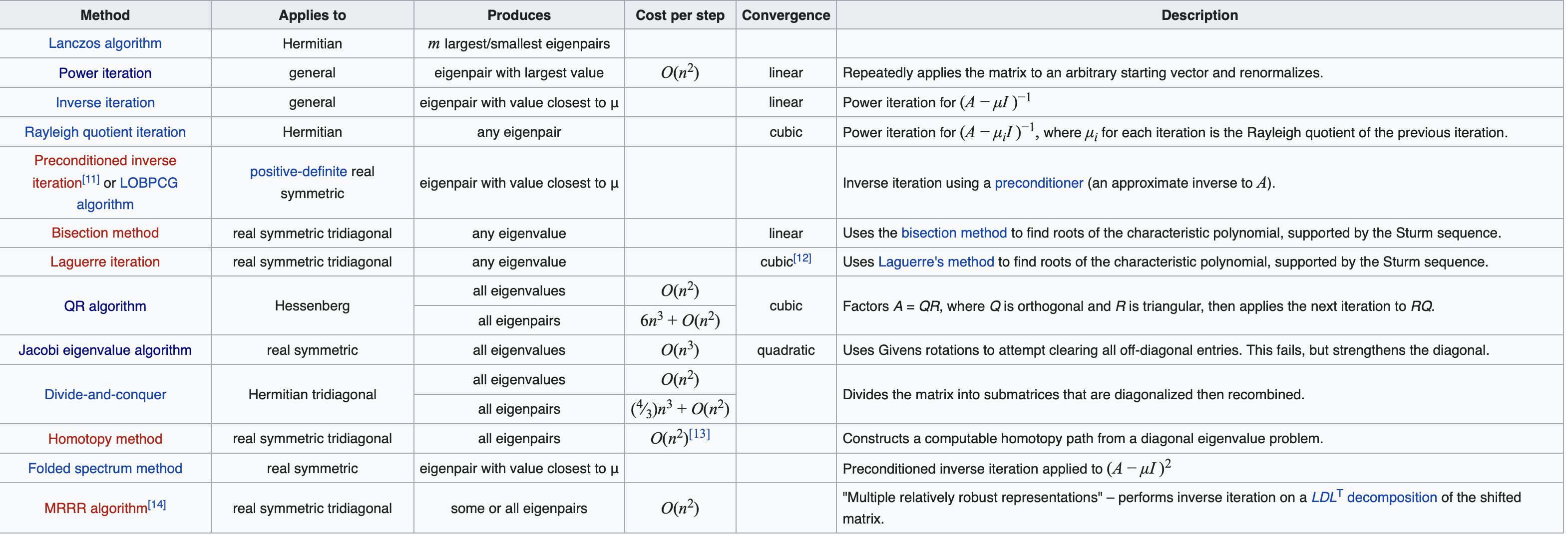
4. Methods to calculate eigenvalues and eigenvectors

   • Old-school method:

     Solve characteristic equation $A - \lambda \cdot I = 0$ —> $det(A - \lambda \cdot I) = 0$.

     Example

     \[A = \begin{bmatrix} 2 & 2 \\ 1 & 3 \end{bmatrix}\] \[det(A - \lambda \cdot I) = 0 \\ \Rightarrow (4 - \lambda) \cdot (1 - \lambda) = 0 \\ \Rightarrow \lambda = 1 \space, \space \lambda = 4\]

     Finally, we have 2 eigenvectors: $\begin{bmatrix} 1\ -1 \end{bmatrix} \space , \space \begin{bmatrix} 1 \ 2 \end{bmatrix}$.

   • Others

     

Source: Wikipedia.

1. Experiment on longterm behaviors and power iteration method (Include code).

2. A cool things in finding eigenvalues.
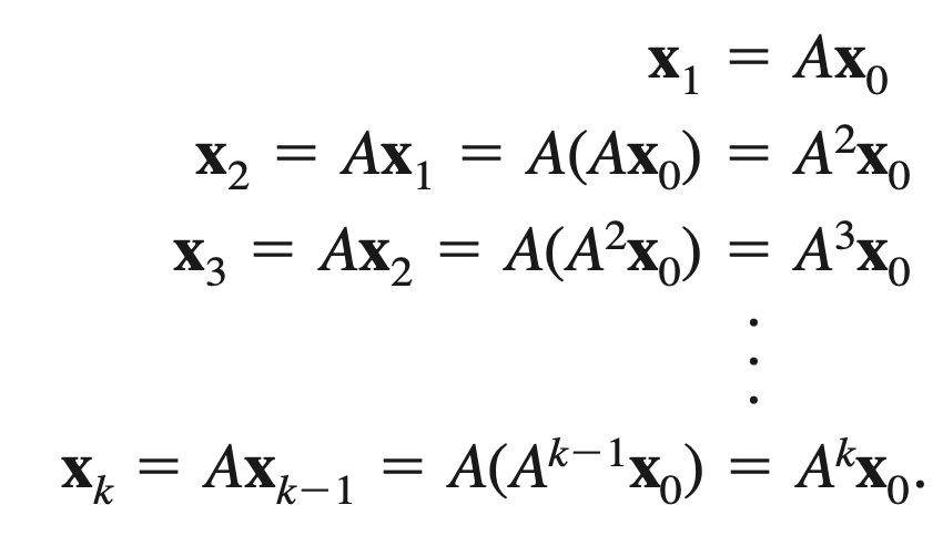
   • Consider a model with a linear transformation of $v_{output}= A^n \cdot v_{input}$ (Applying multiplication of A into vector V, of n times).
   • We initialize model with a random 5x5 matrix A whose elements follow a Gaussian distribution, mean = 0, variance = 1.

    ximport numpy as np
    import matplotlib.pyplot as plt
   
    #initialize matrix A
    np.random.seed(8675309)
    A = np.random.randn(5, 5)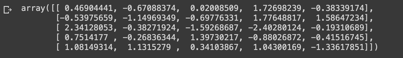
   

   

    #initialize vector v
    v_in = np.random.randn(5, 1)
    norm_of_v = [np.linalg.norm(v_in)]
   

    #Implement n = 100
    n = 100
    for i in range(1, n):
        v_in = A.dot(v_in)
        norm_of_v.append(np.linalg.norm(v_in))
   
    plt.plot(norm_list)
    plt.xlabel("Iteration")
    plt.ylabel("Value")
    plt.show()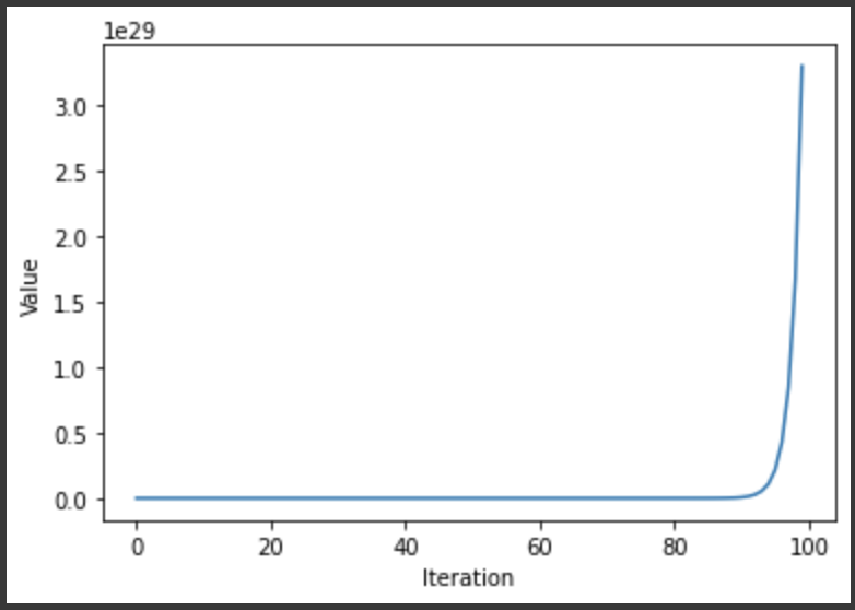
   

   

   —> The norms just increase significantly.

   —> Because we apply A n times in the vector V, therefore, the norm of the vectors keep stretching enormously.

   If we take a list of quotient, a pattern will show up.

    quotients = []
    for i in range(1, 100):
        quotients.append(norm_of_v[i] / norm_of_v[i - 1])
   
    print("Approxiamtion for eigenvalue is", quotients[-1])
    plt.plot(quotients)
    plt.xlabel("Iteration")
    plt.ylabel("Value")
    plt.show()
   

   

   

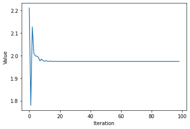
   —> The ratio ocillate in a stable value (about 1.98), which is also the largest eigenvalue, called “singular value”. —> this is so called “rate of convergence”

   If we use the numpy library to compute the eigenvalues (cross check):

    eigs_vals = np.linalg.eigvals(A).tolist()
    eigs_vals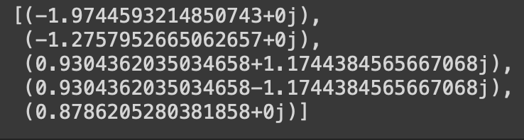
   

   

   —> This results contain many complex numbers. This can be thought of stretching or rotating.

   —> Taking the Euclidean norm of all the values (both real and complex number) —> we obtain the stretching factors (eigenvalues) with numpy.

    norm_eigs = [np.absolute(x) for x in eigs_vals]
    norm_eigs.sort() #sorting to be more easy to visualize
    print(f'norms of eigenvalues: {norm_eigs}')
   

   

   The biggest value is 1.9744593214850743 —> this is so important that we can call it “principle eigenvalue”, which is so close to our approximation (1.9744593214851518).

3. Power Iteration method

   a. Dominant Eigenvalues (Singular Value)

   Definition: Let $\lambda_1, \lambda_2, \lambda_3, …. \lambda_n$ be the eigenvalues of N x N matrix A. $\lambda_1$ is called the dominant eigenvectors of A if:

   \[|\lambda_1| > |\lambda_i|, i= 2, 3,... n\]

   b. Approach to power method.

   • As witness from the implementation above, we can obtain how to use this iterative method on finding eigenvalues.

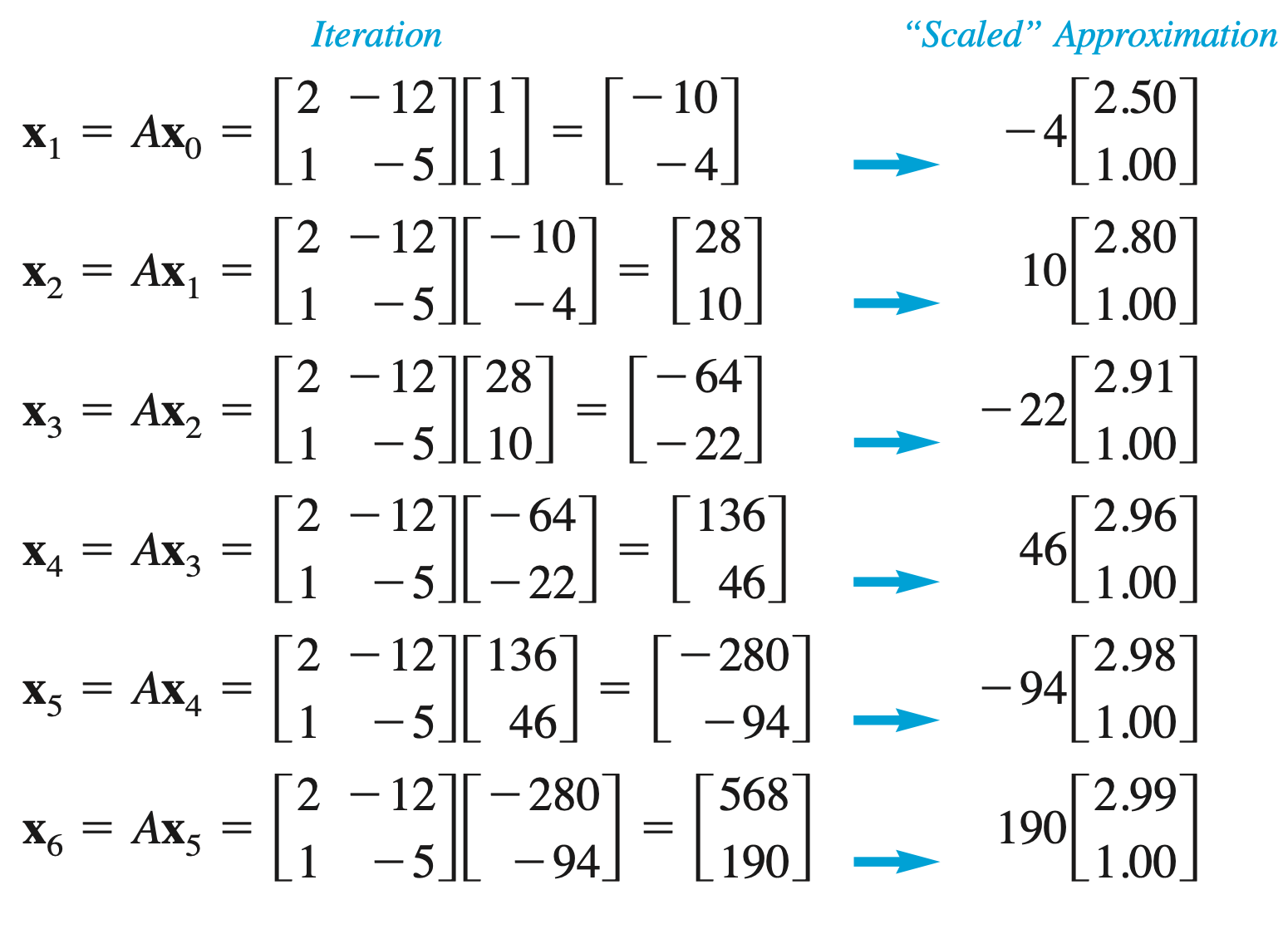
   • Simply, we will apply dot product of an original matrix A to a vector V and continue apply A to the result A.v:

     

     • For the large number of k —> we can obtain good approximation.
     • Example: We have matrix A and vector x.
     \[A = \begin{bmatrix} 2 & -12 \\ 1 & -5 \end{bmatrix} \\ x_0 = \begin{bmatrix}1 \\ 1 \end{bmatrix}\]

     • Then we can obtain:

       

   c. Rayleigh quotient to get the eigenvalue

   Definition: If x is an eigenvector of a matrix A, then its corresponding eigenvalue is given by

   \[\lambda = \frac{A\cdot x}{x\cdot x}\]

   Proof:

   We have: $A\cdot x = \lambda \cdot x$

   We can write:

   \[\frac{A\cdot x \cdot x}{x \cdot x} = \frac{\lambda \cdot x\cdot x}{x\cdot x} = \lambda\]

   For the above example: we have

   

   

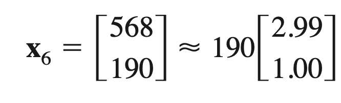
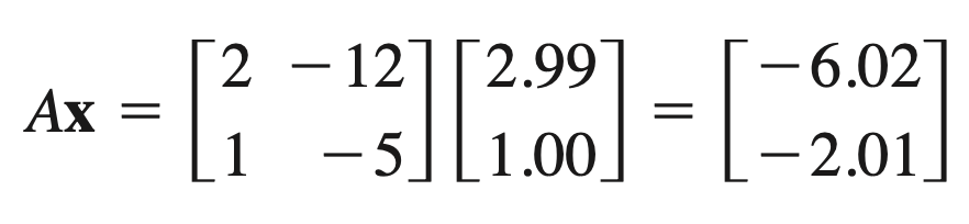
   So, A.x. x = -20.0 and x. x = 9.94 —> $\lambda = \frac{A\cdot x \cdot x}{x \cdot x} = \frac{-20.0}{9.94} = -2.01$

   d. Rate of Convergence of Power Method

   We have matrix \(A = \begin{bmatrix} 4 & 5 \\ 6 & 5 \end{bmatrix}\) has eigenvalues \(\lambda_1 = 10, \lambda_2 = -1\)

   —> The ratio is \(\frac{\lambda_2}{\lambda_1} = 0.1\)

   e. Complexity: O(n^2)