- Overview.
- In linear regression, we face with prediction problem, which is related to linear data.
- Taking an example, building a system to decide a student is fail or pass the exam based on the hour he/she spent on studying.
Like this:
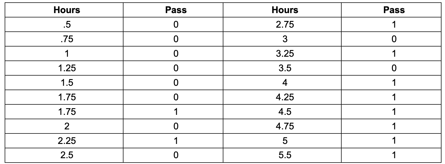
- At first glance, the output is clearly just 1 or 0 (1 means pass and 0 otherwise) —> this is so-called “binary classification”.
-
Then, based on the output, we can represent in graph with 2 regions located in line y = 1 and y = 0. Like this
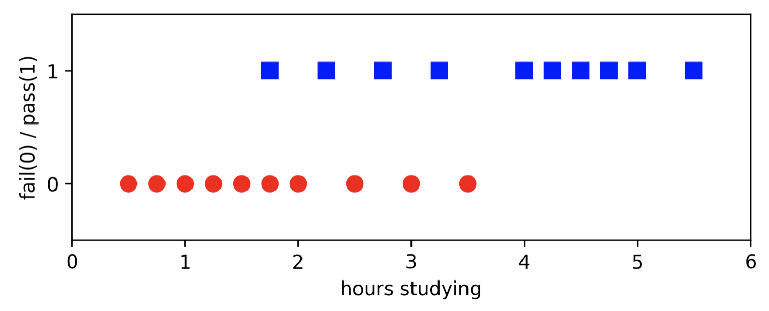
- With this in mind, we can obviously use linear regression to draw a fitting line to the data and it may give the correct answer if we luckily have nearly zero noise. In other word, assume that there is a student spend very little time on studying but gain a better result than one who take a lot of time to study and suddenly fail the exam. Or, sometimes, someone cheated —> linear may give the wrong answer when that annoying point happens.
- However, it is not necessary to be a line, it can be a parapol or a very strange function as long as we are able to calculate it and as long as it can fit data well.
-
Clearly, with 1 means pass and 0 means fail. So, 0.5 is a boundary between two regions, right. Simply, 2 horizontal lines will fit data well, our job is to find the connector between two horizontal lines.
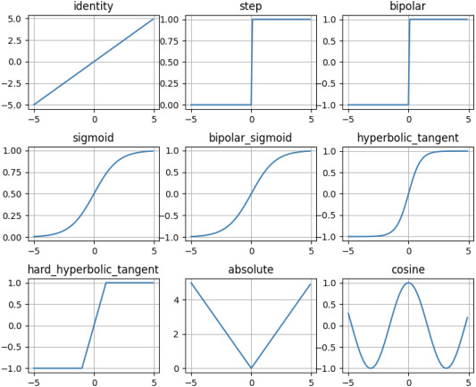
In the given list of activion function, we can chooe the binary step (row 0, column 1), in which we change (-1, 1) to (0, 1). However, the straight line connects points (1, 0), and (0, 1) will cause problem. Assume that some students have 0 time or 1 hour of studying and still pass the exam, which is a dream reality 😂.
However, to be serious the step function can not be used because of “hard threshold”
In conclusion, using sigmoids or something like that in row 1 of the picture is the best (and also more beautiful).
- For a very basic and very good to fit, we use original sigmoid function with properties:
- Constant and differentiable, bordered by 2 lines: y = 1 and y = 0 —> (0, 1).
-
The number of points which are far from 0.5 on the leftside will approach to 0 and vice versa (approach to 1). Which is
\[\lim_{x \rightarrow -\infty} f(x) = 0 \\ \lim_{x \rightarrow \infty}f(x) = 1\] - In fact, scientists did the hard one, they do find a function like that:
—> this is so-called “sigmoid function”
- Loss Function
- In fact, try to decide a student fail or pass the exam is quite hard, because there are number of ways can be happened to one person or a lot of people. For example, a student can be very smart and is required less time to pass the exam, otherwise, a really bad student can not fulfil the exam despite trying hard. Or sometime luck involves, some students can pass the exam smoothly, in addition, cheating is also a way to make our prediction harder. With the being said, the data is not linearly separable, which means in our assumption, we can coldly calculate the probability to decide whether student can pass the exam based on the quantity of reviewing time (and may be other elements, too).
- Probability is not always right for reality but at least when many elements involved it can be more precise and also people can not blame the computer scientist for that 😂
- In an easy way, to calculate probability, we witness that there are 2 classes (pass: 1 and fail: 0), let f be the probability of a point x lying in class 1 and 1-f is the probability that x lying in the class 0. In other word, f is our function (function f whose output is a probability of x, y, z,… in the coordinate), whose domain is (0, 1). We can write in the form of conditional probability:
- Hence, our goal is to find parameter “theta” such that f(theta^T * xi) is close to 1 with the point belongs to class 1 ($x_i \in [0.5, 1]$) and is close to 0 with the point belongs to class 0 ($x_i \in [0, 0.5]$).
-
Let $z_i$ denote $f(\theta^Tx_i)$, we can write this above messy formula in one clean line of formula using a little bit of changing and rearranging:
\[P(y_i|x_i, w) = z_i^{y_i}(1-z_i)^{1-y_i}\] -
In this formula, we can understand that x and y are random variables. For a training set: $X = [x_1, x_2, …, x_{N}] \in R^{len(x) \times N}$and $y = [y_1, y_2,…, y_{N}]$ —> $P(y X; \theta)$ (X and y are also random variables). -
For every element in X, it is clear that they are independent and happen at the same time (imaging a bunch of students, they do the exam independently together). According to the multiplication rule for the probability of the coincidence, we can obtain loss function:
\[P(y|X; \theta) = \prod_{i=1}^{N}P(y_i|x_i;\theta) = \prod_{i=1}^{N}z_i^{y_i}(1-z_i)^{1-y_i}\] -
From probability class, we all know that $P(y X; theta)$ is a conditional probability in which we specified the likelihood or the probability that y = 0 or 1 happens with the given X and theta (X parameterized theta). If the student belong to class 1, we want P for y = 1 is super high and P for y = 0 is deeply low and vice versa. - With that in mind, we are likely to maximize that probability for loss function
- Optimization for Loss Function
-
Based on our idea in the previous section, obtain our goal is to find parameter theta that maximize P:
\[\theta = \argmax_{\theta}P(y|X;\theta) = \argmax_{\theta} \prod_{i=1}^{N}z_i^{y_i}(1-z_i)^{1-y_i}\] -
For the given optimization problem like that, it is quite difficult to find the optimal point. One simple approach is to take the logarithm of the right handside. So, the product can become the sum, which is easier to compute. One more step (optional) is to put the minus sign in front of the log function —> maximize become minimize, which is quite familiar.
\[L(\theta) = - \log P(y_i|X; \theta) = - \sum_{i=1}^{N}(y_i\log z_i + (1-y_i)\log (1-z_i)) \tag{1}\]- The right hand side is so-called “cross entropy”, which is used to calculate the distance (error) between 2 distribution.
- Note: logarit here can be natural log (ln), which is more popular than normal logarit.
- Tip: Using SGD (stochastic gradient descent) or mini batch to optimize this can produce a good result in a short amount of time.
-
Firstly, find the derivative at one point $(x_i, y_i)$ is $L(\theta;x_i, y_i) = -(y_i\log z_i + (1-y_i)\log (1-z_i))$
\[\frac{\partial L(\theta;x_i,y_i)}{\partial \theta} = \frac{z_i-y_i}{z_i(1-z_i)}\frac{\partial z_i}{\partial \theta} \tag{2}\] -
Then, let $s_i = \theta^Tx_i, \space s’ = x_i$, applying chain rule
\[\frac{\partial z_i}{\partial \theta} = \frac{\partial z_i}{\partial s} \cdot \frac{\partial s}{\partial \theta} = \frac{\partial z_i}{\partial s_i} x_i \tag{3}\] -
Subtitute (3) into (2), obtain:
\[\frac{\partial L(\theta;x_i,y_i)}{\partial \theta} = \frac{z_i-y_i}{z_i(1-z_i)}\frac{\partial z_i}{\partial s_i} x_i\ \tag{4}\] - To continue the next important step, we may need to go back to the first thing ever:
- We have sigmoid: $\sigma(s) = \frac{1}{1+ e^{-s}}$
- Gradient of sigmoid: $\sigma’(s) = \sigma(s)(1-\sigma(s))$
- Output of logistic regression model denoted by: $z_i = f(\theta^Tx_i)$ and $s_i = \theta^Tx_i$
—> The connection between 3 views above is quite clear. To be easy to understand, we obtain, $z_i = \sigma(s_i) = \sigma(\theta^Tx_i)$
-
Hence, the derivative at $(x_i, y_i)$:
\[\frac{\partial z_i}{\partial \theta^T x_i} = \frac{\partial \sigma(s_i)}{\partial s_i} = \sigma(s_i)(1-\sigma(s_i)) = z_i(1-z_i) \tag{5}\] -
Then, subtitute (5) to (4), obtain:
\[\frac{\partial L(\theta;x_i,y_i)}{\partial \theta} = (z_i-y_i )x_i\]Clean, fresh and very very beautiful right 😂
-
Now, applying SGD for the given derivative formula:
\[\theta_{i+1} = \theta_i + \eta\cdot(z_i - y_i)x_i\]- The plus size is because we do not use the minus in (1), so we need to maximize, means that we use gradient ascent and otherwise, with minus sign in (1), we will minimize by gradient descent.
- Finally, we have all materials are necessary to build our model. Let’s take a quick look in how sigmoid function is created.
- We have: $\frac{\partial z_i}{\partial s_i} = z_i(1-z_i) \Leftrightarrow \frac{\partial z_i}{z_i(1-z_i)} = \partial s_i \Leftrightarrow (\frac{1}{z_i} + \frac{1}{1-z_i})\partial z = \partial s_i$
- Take the integral (note that log here is ln)
-
Solving that equation:
\[z_i = e^{s_i} (1 - z_i) \Leftrightarrow z_i = \frac{e^{s_i}}{1 +e^{s_i}} = \frac{1}{1 + e^{-s_i}} = \sigma(s_i)\]
-
Code:
  def sigmoid(s):
      return 1/(1 + np.exp(-s))

  def gradient(X, y, z):
      return (y - z) * X

  def update(X, y, theta, eta, iter):
      # batch size = 1
      n_features = X.shape[1]
      train_size = X.shape[0]
      train_loss = []
      for epoch in range(iter):
          temp = np.random.permutation(n_features)
          for i in temp:
              xi = X[:, i].reshape(train_size, 1)
              yi = y[i]
              zi = sigmoid(np.dot(theta.T, xi))
              theta = theta + eta * gradient(xi, yi, zi)
              train_loss.append(zi/train_size)
      return theta, train_loss
-
- Discussion
- Main disadvantage of Logistic Regression is all data must be independent (imaging that a group study can beat the correctness of this algorithm).
- There is number of way to compute for loss function: absolute value (L1), mean square error (L2), Hubber,… Each kind of loss has its own benefits and drawbacks.
- Reference
Blog and stuffs