- Overview
- Linear regression is an interesting thing in statistic, which we can compute the future value of a function by feeding it with huge number of data (the spreading of data is linear).
-
In other words, the more “linear” data is, the more precise we can predict.
- Example:

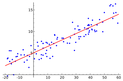
- It is easy to see that the data is increasing. Despite some weird behavior, it is generally increasing (or sometimes decreasing 😂)
- So, for linear data (just simply call by that name), we can easily witness the future by our eyes, and so does machine.
- Can take the housing problem as an example, suppose we want to evaluate a house with N square meters (area). We all know that the larger the house is, the more expensive it is. Therefore, we can easily predict (or evaluate) the price of a house based on its area.
- Machine can learn this, what we need is an algorithm which can produce the nearly precise output, after eating a bunch of data in reality.
- Easily, just simply draw a line which can fit the data in the scatter graph well.
-
Like this:
- So, find a line in a graph == find a linear function
- Luckily, we know in 2D space, the function is: $y = a \cdot x + b$ (in which a is slope, b is y intercept — it is general math stuff).
-
In multidimensional space: $y = a_1 \cdot x_1 + a_2\cdot x_2 + ….. + b$ (depend on dimension, this can be line - 2D or plane - 3D or hyperplane - xD).
Here, b is also called bias value. We all know in linear algebra, the line is perfectly start from the origin of the 2D coordinate O(0, 0), but in reality, there is always a bias value cause the line a little bit far from the origin.
In the picture above, y-intercept (or bias) is 5.
- With that being said, our work now is much simpler, just finding the most suitable line fit all the data. Question is how can we draw such a line.
- For a data point ( a small dot in the graph), it is very intuitive that the distance from an arbitrary line to that dot is smallest when the dot is on the line.
- Assume that we have a bunch of dot which is not standing on a line together, means that we can not put all the points in a line together, because they are not straight.
- In fact, it is not necessary that all the points must lie in a line, the goal is the nearly fitting line, which have the distance from that line to the point is the smallest (nearly 0).
- With that idea, we all know that in a 2D dimensional space, the distance between a point and a line is just simply calculating Norm (using Euclidean Norm here).
-
Therefore, we obtain loss function (loss here means “error”, because the distance from point to fitting line is error, we want to minimize the error).
\[L(w) = \frac{1}{2} \cdot \sum^N_{i=1} (y_i - \bar{X}_i \cdot w) ^2\]- N is number of data points (number of blue dot in the above graph).
- Inside the sum is the Error formula. Because we assume the perfect line is starting from the origin, which have function: y’ = w . X and the reality line is y = ax + b —> we just simply implement: error = y - y’, it may be negative, we must use square or absolute value. However, we have to take the derivative afterward, so just use square (or can say “Euclidean Norm).
- X bar is a vector with multiple columns, in multidimensional data, X bar is a matrix with corresponding columns and rows.
-
1/2 is a scalar for easy to compute, because in reality, the dataset is massive. When taking the derivative, the 0.5 scalar is automatically reduced.
Another way to represent loss function:
\[L(w) = \frac{1}{2} \cdot \|y - \bar{X} \cdot w \|_2^2\]
- Now, our work is clear, just find the minimum value for the Loss Function.
- Normal Equation
- In Vietnam, we learn in grade 12th about the application of derivative, if we want to compute the min value of a function, just simply take the derivative, let the derivative = 0, solve the function and we all know the max and min value.
-
However, in many problems, the function is hard to find the derivative or hard to compute the value for equation: derivative = 0. Luckily, in linear regression, it is possible.
By using partial derivative, obtain:
\[\frac{\theta L(w)}{\theta w} = \bar {X}^T \cdot (\bar{X} \cdot w - y)\]- For the derivative = 0, obtain:
-
So, the equation have solutions if the vector / matrix multiplication in the lefthand side is invertible (non singular). We obtain the solution for w:
\[w = (\bar{X}^T \cdot \bar{X})^{-1} \cdot \bar{X}^T \cdot y\]The complex thing: $(\bar{X}^T\cdot\bar{X})^{-1}\cdot \bar{X}^T$ is called “Pseudo inverse” (just the name). And the equation above is called “Normal Equation”.
- So, for this intuitive idea of normal equation is used to solve linear regression problem when we are able to compute the derivative and calculate the derivative = 0.
- Disadvantage:
- Work well with small number of features, when the features scale bigger, the normal equation is slow (features are different from data point, features mean the category of data, for example, for house price prediction, features are area, number of bedrooms, quality of neighborhood and so on).
- The X Transpose * X must be invertible, otherwise, must use regularization to handle
- Time complexity is O(n^3) where n is number of features.
- Batch Gradient Descent
- Batch Gradient Descent is a technique, it is also the original gradient descent (I think).
- Firstly, “Gradient” means something related to derivative. In function y = ax + b, a is slope, obviously, when taking the derivative, x & b are reduced, a remained will represent for the trend of the linear function (increase or decrease). In multivariable function (many X), slope is called “gradient” —> in general case of slope, obtain gradient.
- Secondly, “Descent” means go backward (or go reverse), in a function, its shape like a mountain, we want to go to the valley, so we must go down (descent).
- Finally, “Batch” doesn’t matter here, because it just represents what kind of Gradient Descent (GD) it is.
- Together, we obtain “Gradient Descent” means a man called “Gradient”, he go downward to reach the valley of a mountain-like function. In other word, it is just simply we take the initial place to start (may be on top of the mountain), take the derivative and minus it 😂 to go backwards.
-
To be more specific:
\[x_{t+1} = x_{t} - \eta \cdot \frac{\partial f(x)}{\partial x}\]Firstly, we can see here, it is easy for us to do this as a programmer 😉, obviously, a for loop might help!
Secondly, in detail, the complex part is just the derivative of the loss function, which we consider here is linear regression.
Thirdly, the “eta” symbol is called “learning rate”. Clearly, machine is not human, it can not walk on it own, we need to set the pace of its walk (to the valley), the pace also reflects the speed of this algorithms. If learning rate is too big (like moving a big step downward), the algorithm will never give precise answer (because, once again, it is a machine, not human). And vice versa, too small —> too slow to reach the valley (or even never reach).
—> Overall, imagine a man called “Loss”, he carried a bunch of package on his body, he want to go down to the valley as soon as possible, so he take off all the necessary things to obtain a lightweight body (called “gradient”), we set for him an initial place, which is x0, and require him to go with, say, 0.1 kilometer at each step (each loop).
—> In conclusion, learning rate eta is too low —> slow, too high —> never reach optimal point (valley). Remark:
- In the formula, we update x1 by let x0 - eta * derivative of loss function and so on for other values —> do it in one loop with identified iteration (we set iteration).
- For different x0, we often get nearly the same solution
-
Example:
$f(x) = x^2 + 5 \cdot sin(x)$
$\Rightarrow f’(x) = 2 \cdot x + 5 \cdot cos(x)$
  import numpy as np
  import matplotlib.pyplot as plt

  def Grad(x):
    return 2*x+ 5*np.cos(x)

  def Cost(x):
    return x**2 + 5*np.sin(x)

  def GD(x_0, weight):
    res = []
    for i in range(100):
      x_0 = x_0 - weight*Grad(x_0)
      res.append(x_0)
      if abs(Grad(x_0)) < 1e-3:
        break
    return (res[-1], i)
Testing:
  print(GD(-5, 0.1))
  print(GD(5, 0.1))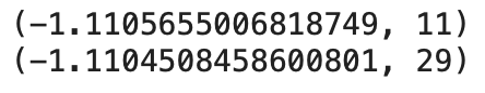
—> the minimum value obtained after 11 loops (x_0 = -5). The same with 29 loops (x_0 = 5)
Plot:
  x = np.arange(-5, 5, 1) #x_initial = -5
  f = Cost(x)
  point_x = GD(-5, 0.1)[0]
  point_y = Cost(point_x)
  print(mark)
  plt.plot(x, f)
  plt.scatter(point_x, point_y)
  plt.xlabel("x")
  plt.ylabel("f(x)")
  plt.show()
-
For linear regression:
  def Loss(weight):
  	return 0.5/N * np.linalg.norm((y - np.dot(X, weight))) ** 2
  def Gradient(weight):
  	(1 / N) * np.dot(X.T, ( np.dot(X, weight) - y))
  def Update(weight_init, eta, iteration):
  	train_size = len(X)
  	weight = weight_init
  	for i in range(iteration):
  		loss = Loss(weight)
  		weight = weight - (eta / train_size) * gradient(weight)
  		loss /= train_size
  	return weight, loss
—> weights are the output of the function.
- Advantage:
- Easy to compute (use the power of machine), high adaptability.
- Matrix of dataset doesn’t have to be invertible, square,…
- Complexity: O(n^2)
- Stochastic Gradient Descent (SGD)
- In reality, the dataset is huge, and batch GD (or traditional GD) may go slow. Therefore, a little update is necessary to improve the speed of convergence of the algorithm but still remain the value of weight found.
- SGD is a kind of GD but use only one datapoint to represent for a huge datasets (note: one point each time).
-
So, the formula for 1 point is:
\[L(w, x_i, y_i) = \frac{1}{2}(x_i^Tw - y_i)^2 \\ \Rightarrow L'(w, x_i, y_i) = x_i^T(x_iw-y_i)\] -
To be easier, just using 2 loops, each epoch (outside loop) runs n times (n is number of datapoints), means that each epoch, our algorithm will take a look to a whole data based on 1 datapoint (given in random order). During an epoch, shuffle data of X parameter is require.
def stochastic_gradient_descent(X, y, w, eta, iter): # batch size = 1 train_loss = [] temp = np.random.randint(N) for epoch in range(iter): np.random.shuffle(X) for i in range(N): xi = X[temp : temp + 1] yi = y[temp : temp + 1] l = (np.dot(xi, w) - yi)**2 grad = 2* xi.T.dot(np.dot(xi, w) - yi) w = w - (eta) * grad train_loss.append(l[0][0]/N) return w, train_loss - Advantage:
- faster in the speed of convergence —> can find the optimal point quickly.
- require a small number of iteration.
- Disadvantage: sensitive with noise and the loss function is not as beautiful as traditional GD.
- Mini-batch Gradient Descent
- The idea is quite the same with SGD, however, instead of taking only one datapoint to represent a bunch of elements each time, we will use a set of points.
-
Now the formula is
\[\theta = \theta - \eta\nabla_{\theta}L(\theta, x_{i, i+n}, y_{i, i+n})\]- n is number of batch size = number of points we want to take. A good tip is just taking a number that is a perfect square root i.e 2^2, 2^3, 2^4,….
- x is the data from i to i+n.
- Like SGD, shuffle X is required to have a better results 😂
def minibatch_gradient_descent(X, y, w, eta, iter, batch_size): train_loss = [] for epoch in range(iter): np.random.shuffle(X) for i in range(0, features, batch_size): X_i = X[i:i+batch_size-1] y_i = y[i:i+batch_size-1] l = (np.dot(X_i, w) - y_i)**2 grad = 2* X_i.T.dot(np.dot(X_i, w) - y_i) w = w - (eta) * grad train_loss.append(l[-1][-1]/N) return w, train_loss - Advantage:
- Faster in speed
- Small number of iterations
- Useful with a huge number of data.
- Disadvantage: loss is not beautiful 😂
- Reference
Blog and stuffs