• Basic operation: operation which is used most of the time. For example in linear search, “==” operation is a basic operation.

• What is algorithms? An algorithm is a finite sequence of precise instructions for performing a computation or for solving a problem. (according Rosen in his textbook).

• If you want to develop an algorithm, which properties should you consider?
  1. Input —> values from a specified set.
  2. Output —> a set of input values produces a set of output values.
  3. Definiteness —> steps of an algorithm must be defined precisely.
  4. Correctness —> correct output values for each set of input values.
  5. Finiteness —> produce the desired output after a finite steps.
  6. Effectiveness —> perform each step in a finite amount of time.
  7. Generality —> applicable for all problems of the desired form.
• Runtime: number of execution of basic operator in a specific program. For example in linear search, runtime is N because it execute basic operation “==” N times (N is length of array).

• Asymptotic notations are the mathematical notations used to describe the running time of an algorithm when the input tends towards a particular value or a limiting value.
• We consider here the the very large input size (which is nearly to infinity) —> therefore we called it “Asymptotic”. For example, consider the function:

—> If we try sketching this function, we can obviously witness that, with x become larger and larger (x → inf). This function seem to be closer to it original version $f(x) = x^2$, in other word, the input size x increase bigger and bigger, 6 times x, plus 100 x and plus 300 will make no meaning. Fun fact: How can we multiply infinity to 6 after that plus 100 multiply infinity and plus 300 to the infinity value 😅?

—> Therefore we automatically remove 6, 100x and 300. Obtaining runtime = x^2 clearly and briefly.

• In order to calculate effectively the efficiency of an algorithm, it is necessary for us to have 3 cases:
  1. Best case.
  2. Average case.
  3. Worst case.
• For example in bubble sort:
  • when the input array is already sorted, the time taken by the algorithm is linear i.e. the best case.
  • when the input array is in reverse condition, the algorithm takes the maximum time (quadratic) to sort the elements i.e. the worst case.
  • when the input array is neither sorted nor in reverse order, then it takes average time. These durations are denoted using asymptotic notations.

  (according to programmiz).

1. Big O notation.

   Let f and g be functions from the set of integers or the set of real numbers to the set of real numbers. We say that f (x) is O(g(x)) if there are constants C and k such that:

   \[|f(x)| \leq C \cdot |g(x)|\]

   In other word, the growth rate runtime is represented just like a function, Big O is an upper-bound of that function.

   Imaging that you have 1 billion dollar in your bank account, however, you spend money for your life is always less than 1 billion dollar. Means that 1 billion dollar is your upper limit of your budget.

   —> Big O measures the worst case of the algorithms.

2. Big Omega notation.
   • The same with Big O.

   Let f and g be functions from the set of integers or the set of real numbers to the set of real numbers. We say that f (x) is O(g(x)) if there are constants C and k such that:

   \[|f(x)| \geq C \cdot |g(x)|\]

   In other word, the growth rate runtime is represented just like a function, Big O is an lower-bound of that function.

   —> Big Theta measures best case of the algorithms (which we prefer).

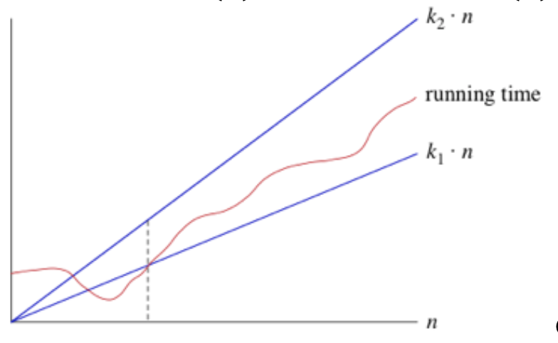
3. Big Theta notation.
   • It is easy to guess, big Theta is the average case of the algorithms.
   • For example, with $\theta(n)$, means that when n is big enough, runtime is smaller than k1 multiply n and bigger than k2 multiply n (see picture below).

   

   

• Non-recursive:
  1. Identify basic operation.
  2. Measure how many times that basic operation execute.

  3. Make it into a “Closed form” (discrete math stuff) —> in case there are many basic operation, we take the max of the runtime of those basic operations.

     Note: Suppose that f1(x) is O(g1(x)) and that f2(x) is O(g2(x)). Then (f1+f2)(x) is

     \[O(max(|g_1(x)|, |g_2(x)|))\]
• Recursive:
  • Use recurrence relation: just look at the problem and use the discrete math knowledge. You can google it!.
  • Solving the recurrence relation —> we can use some beautiful formula for linear recurrence relation or using generating function. You can also google it! (because it belong to discrete math).
  • Another option: we can use naive approach: backward substitution.

1. Master theorem.
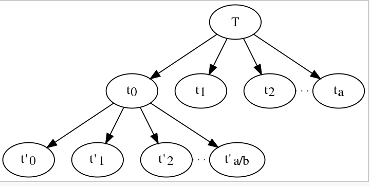
   • We have the pseudo code for our recurrence relation:

   procedure P(input x of size n): if n < some constant k: Solve x directly without recursion else: Create a subproblems of x, each having size n/b Call procedure p recursively on each subproblem Combine the results from the subproblems

   • The master method is a formula for solving recurrence relations of the form:
   \[T(n) = a \cdot T(\frac{n}{b}) + f(n)\]
   • Note that f(n) is the time to create the subproblems and combine their results in the above procedure.

   • T(n) has the following asymptotic bounds:

     1. If f(n) = O(nlogb a-e), then T(n) = Θ(nlogb a).

     2. If f(n) = Θ(nlogb a), then T(n) = Θ(nlogb a * log n).

     3. If f(n) = Ω(nlogb a+e), then T(n) = Θ(f(n)) (e > 0 is a constant)

   • To be more clear, we based on the asymptotic notation, the recursive method can be executed as follow:

   

   • means that, each time we solving a subproblem of a bigger problem. For example:

       int Fibonanci(int n) {
       		if (n == 0) return 0;
       		else if (n == 1) return 1;
       		else return Fibonanci(n-1) + Fibonanci(n-2);
       }
     

   • In Fibonanci code, we use the recurrence relation: T(n) = T(n-1) + T(n-2), which means each time: T will be divided into T(n-1) and T(n-2). For T(n-1) will be divided into T(n-2) + T(n-3) and so on. The same with T(n-2).
   • According to Master theorem,
     1. each time we create subproblem from a bigger problem, the cost increase about a value, in the Fibonanci, it increases approximately 2^n times (google it for more precise value $n^{ log_b(n)}$). If it increases at a certain factor (like 2^n but it is not in our case for Master theorem 😅 sorry), therefore, the value of f(n) will become polynomially smaller than $n^{ log_b(n)}$. Thus, the time complexity is oppressed by the cost of the last level. (like $n^{ log_b(a)}$).
     2. The same as 1, if the cost for creating is nearly equal, f(n) will become equal to $n^{ log_b(n)}$, then value will be total number of level (or step of execution) (like $n^{log_b a} * log(n)$ )
     3. The same as 1, if the cost for creating is nearly reduced, f(n) will become bigger than $n^{ log_b(n)}$, then value will be f(n).
   • Example: Solving:
   \[T(n) = 3 \cdot T(\frac{n}{2}) + 2\cdot n \\ \rightarrow log_b(a) = log_2(3)= 1.58 < 2\]

   —> in case 3 above, T(n) = f(n) = $\theta(n)$

Sorting and Searching.

1. Binary Search.
   • Applied for sorted array.
   • Complexity: O(log n) (for worst and best case).
   • Space: O(1)
   • Divide and conquer algorithms: The main thing is find middle element and compare.
   • Can use recursive or iterative method.
   • Notice: we use formula: mid = low + (high - low)/2 instead of mid = (low + high) to prevent sum overflow. If there are 2^31 - 1 (or more) elements in array, the program will quickly return -1 😂

    // iterative method:
    int Iterative_Binary_Search(int arr[], int low, int high, int value) {
        while (low <= high)
        {
            int mid = low + (high - low)/2;
            if (arr[mid] == value) {
                return mid;
            }
            if (arr[mid] < value) { low = mid + 1; }
            else { high = mid - 1; }
        }
        return -1;
               
    }
   
    // recursive method
    int Recurvise_Binary_Search (int arr[], int low, int high, int value) {
        if (high >= low) {
            int mid = low + (high - low)/2; 
            if (arr[mid] == value) {
                return mid;
            }
            if (arr[mid] > value) {
                return Binary_Search(arr, low, mid - 1, value);
            }
            return Binary_Search(arr, mid + 1, high, value);
        }
        return -1;
    }
   

2. Interpolation Search.
   • Interpolation search is faster than binary search for some special case.
   • Binary Search goes to the middle element to check irrespective of search-key. On the other hand, interpolation search may go to different locations according to the value of the key being searched.
   • The main different here is the formula for mid element.
   • Proof and Formula:

    Let's assume that the elements of the array are linearly distributed.
   
    General equation of line : y = m*x + c.
    y is the value in the array and x is its index.
   
    Now putting value of lo,hi and x in the equation
    arr[hi] = m*hi+c ----(1)
    arr[lo] = m*lo+c ----(2)
    x = m*pos + c     ----(3)
   
    m = (arr[hi] - arr[lo] )/ (hi - lo)
   
    subtracting eqxn (2) from (3)
    x - arr[lo] = m * (pos - lo)
    lo + (x - arr[lo])/m = pos
    pos = lo + (x - arr[lo]) *(hi - lo)/(arr[hi] - arr[lo])
   

   • Can do it in recursive and iterative like binary, just use pos instead of mid.

   —> works better than Binary Search for a Sorted and Uniformly Distributed array.

   • Complexity: O(log(log (n))) (best case), O(n) (worst case — i.e: where the numerical values of the keys increase exponentially).
   • Space: O(1)

   —> consider the elements in array when using Interpolation Sort.